Quiz 2

1. Rank order the ten most populous countries of the world. [6 points]
1) China
2) India
3) United States 
4) Indonesia
5) Russia
6) Brazil
7) Pakistan
8) Japan
9) Bangladesh
10) Nigeria 
Open attribute table from cntry02 layer and change POP_CNTRY to sort descending. Answers are under sovereign

2)  15 rivers
Open attribute table from rivers layer and change system to sort ascending. Amazon rivers are listed.

 3) Amu Darya: 52, Syr Darya: 37, total cities: 89

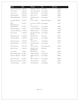
Open attribute table from river layer. Select the two cities. Navigate to Selection and Select by Location. Selection method is select features from and target layer is cities. Source layer is rivers and spatial selection method is features within a distance of source layer. Check apply a search distance, 500 km, then OK. Open attribute table from cities and print screen. Paste in paint because directly pasting on blog slows the computer. Save the images as JPEG and insert image here.

4) 452,300,000
Select by attributes. "CNTRY_NAME" = 'Iran'. Select by location. Target layer is cntry02. The source is cntry02. Spatial selection method within a distance 300 kilometers. Open attribute table from cntry02 layer. Show selected records. Unselect Iran. Look at sum in statistics on POP_CNTR.

5) Most populated: Ethiopia, Least populated: Vatican City
Open attribute table for country layer. Find landlocked and highlight it. Select by attributes. "Landlocked" = 'Y' Open attribute table again and sort descending. Find most and least populous countries.

6) Austria, Bosnia & Herzegovina, Croatia, Czech Republic, Poland, Romania, Slovakia, Slovenia, Yugoslavia.
Open attribute table of cities. Select Veszprem. Select by location. Target layer cntry02. Source layer cities. Spatial selection method is Target layer (s) features are within a distance of the Source layer feature. Apply a search distance 300 Kilometers. Everything else is default. Click OK. Then open attribute table of cntry02. Show selected records. Answers are listed and exclude Hungary.

7) Cameroon, Central African Republic, Libya, Niger. Nigeria, Sudan
 Open attributes table from country layer. Highlight Chad. Select by location. Target layer: cntry02. Source layer: cntry02. Spatial selection method: Target layer features touch the boundary of the source layer feature. Everything else default. Click OK. Navigate to attribute table of country layer. Show selected records. Answers all listed and exclude Chad.

8) 1) Russia (97), 2) United States (93), 3) Thailand (72), 4) Turkey (67), 5) Cote d'Ivory and Poland (both 50)
Open Arctoolbox. Expand analysis tools. click on statistics and click frequency. Input table as cities and frequency field (s) as cntry_name. Click OK. A new table is created. Open new table. Sort frequency descending. Answers are listed. 

9) 2950km + 211km + 599km =  ~3760 km.
Open attribute table of country layer. Find and select Sudan. Use the measuring tool to measure in kilometers the three rivers on Sudan. Estimate the measurements and add the three together.

10) 1) Russia (1516), 2) Canada (1340), 3) United States (743), 4) China (219), 5) Sweden (168)
Same as #8 but input table should be lakes. Use the same frequency tool and choose cntry_name as frequency_field. Click Ok. A new table is created. Open new table. Sort frequency descending. Answers are listed.

11) 1) Canada (443517.19 sq km), 2) United States (196848.52 sq km), Russia (138250.78 sq km), Kazakhstan (70899.672 sq km), 5) Tanzania, United Republic of (53529.613 sq km)
Open attribute table for lakes and go to table options and add field. Name the field. Type should be long integer. Calculate Geometry for the new Area field. Change units to square meters. Under geoprocessing, choose dissolve tool. Input features as lakes. and dissolve_field(s) as cntry_name. Click OK. A dissolved layer will be created. Open attribute table from new dissolved layer. Add new field as before. Name the new field. Type is float to get decimal. change units to square kilometers. Sort descending. Answers are listed.

12)

Open attribute table from dissolved lakes. Navigate to join and relate. Join country layer with the lake dissolves layer. add a new field. Name the field. Use field calculator and find lake dissolves area/ pop_cntry. Edit symbology by changing color ramp and reclassifying the values. 

Los Angeles County Fire Risk Map

     Creating a fire risk map for the Station Fire in Los Angeles County involved several detailed steps. Fire perimeter data and the DEM was provided by the instructor for student convenience. Coordinates for the DEM was changed in order to make the slope model. The coordinates were changed to UTM zone 11 by selecting metric based system project coordinate system and NAD 1983. Therefore, the slope can successfully be created after the hillshade model. The slope was reclassified with appropriate values. The areas with flatter slopes have lower hazard points and areas with steeper slopes have higher hazard points. A steeper slope has a greater risk of catching fire. Additional data on land cover needed to be obtained from the FRAP website. I chose the fuel rank data. Adding the fuel rank data to the map was a simple step. The final component of the fire risk map was combining factors. The slope model and the fuel rank data had to be calculated using the raster calculator. The two were added together to make a summary map. The final product shows the areas at greatest risk in red, orange and yellow. The areas of lowest risk is shown in green. The final product fire risk score proves that the area within the Station Fire has high risk of catching fire because of steep slopes. The fire perimeters of various dates from August to September are included in the map for reference on how the fire grew over time.
     The most difficult problem I encountered during this lab assignment was assigning values for reclassification of the slope. It was difficult to determine the ranges for the classes. Also, I was unsure on how many perimeters I should include in the map. I included one from each date for clarity. I further provided an inset map to indicate where the fire is located in the Los Angeles County. Lastly, it turned out that I did not need to make a slope for my fuel risk layer. This was not required for the raster calculation to make the final product.

Final Project Proposal

Topic: Earthquake hit Virginia, CA and rattled New York, Washington D.C., and others in the east coast.

Methods: Obtain land data from UCLA map share or TIGER website. Make up to 3 maps focusing on the main areas affected by the earthquake. At least one of these maps should show elevation. Also, indicate the areas that were most devastated by the earthquake. Geocode cities and major cities of each state using excel sheets. Add buffers around the earthquake epicenter to show what extent impacted nearby states. Show population data according to each state per province. The earthquake hit today so it is necessary to gather more information and do further research on the subject matter.

Medical Marijuana Dispensaries Policy Brief

     Medical marijuana dispensaries should be at least 1,000 feet away from places where children congregate. It is potentially dangerous to expose children to drug related activities and stores. Children are vulnerable to peer pressure and inappropriate activities. Drugs can affect growth and learning abilities. Drugs can prevent a child from maturing into a adult. Children on drugs will perform poorly in school and have problems socially and physically. Marijuana slows the memory growing process. It is unsafe for children to have access to these types of stores in their neighborhood.
     The map shows various medical marijuana dispensary and elementary school locations in East Los Angeles. Medical marijuana dispensaries are labeled as green points. Elementary schools are labeled as school symbols. Evidently, medical marijuana dispensaries are definitely 1,000 ft away from local elementary schools. Buffers defining the distance from medical marijuana dispensaries are in red.
     Elementary school children will become corrupted. They will not behave properly at home nor at school. As a matter of fact, they will behave poorly. They will start fights with other children. Perhaps, they will join a gang or spend days throughout their lives doing nothing but playing computer games. They are in danger of ruining their futures and health. Smoking at an early age is hazardous to the health. Parents are strongly urged to keep children away from dangerous areas such as areas with medical marijuana dispensaries. Marijuana leads to other more harmful drugs that children are better off not knowing about. Children at a young age need to experience the world by playing with friends and doing educational activities. It is not a bright future for children if they only do drugs and not have a goal in their life. Drugs are not the right toys to play with for children.
     Medical marijuana dispensaries need to ignore the costs involved in keeping their stores away from children. The stores need to collaborate and work together to maintain a safe neighborhood for children. 

References
http://gis.ats.ucla.edu/Mapshare/
http://local.yahoo.com/CA/Los+Angeles/Education/K-12/Elementary+Schools
http://legalmarijuanadispensary.com

Geocoding

     The most interesting topics to read among different news articles are unusual and shocking events. Top stories, whether browsed over the phone or watched on television, are the ones that happen most unexpectedly. Topics range from robbery and murder to natural disasters and war. In conclusion, the topic most read upon are related to tragedy and most likely involve death. Personally, I am fascinated by different criminally related events that take place daily in FOX news or CNN. These types of stories make me wonder how dangerous and illicit the world actually is. Geocoding allows in depth understanding of where certain places are located on a map. In this specific case, homicide has been reported in Los Angeles County for the past month. 

     From July 1st to August 7th 2011, homicide incidents took place in specific locations in Los Angeles County. A total of more than 50 victims have been killed. The case is not always murder. Police officers might have shot and killed a victim. A victim might have been beaten by a group of people and collapsed  miles away from the incident. The most common type of homicide was killing by guns. More than half of the victims were fatally shot. Some of the victims were stabbed. It was shocking to read that some of the victims were elderly, while others were only in their twenties. Bleeding body symbols on the map indicate homicide victims. Evidently, majority of the killings took place near the cities of Inglewood and Hawthorne. There were a few near Long Beach and San Fernando Valley. 

    The map informs potentially dangerous areas of homicide. It can happen to anybody so it is well recommended to take precaution when searching for a new home. This is just a suggestion that the areas with more cluttering of homicide victims are unsafe for family and security. Geocoding homicide addresses onto a map of Los Angeles County showed patterns of killing occurrences in certain areas. On further note, it is difficult to find data shapefiles on locations specifically geared toward the intention of a particular map. Geocoding makes it easy to put points wherever needed. In this case, it helps determine which areas in Los Angeles County are safer than others from homicide incidents. And just to clarify, these homicide locations are the only locations in the Los Angeles County that had victims of homicide during the past month.  

Lab 1 Getting Started with GIS